1 Introduction

This tutorial demonstrates expression-matched gene-set scoring for normalized bulk RNA-seq data. The calculation adapts the control-subtraction principle used by Seurat’s AddModuleScore() to a genes-by-samples matrix: each sample receives the mean expression of its module genes minus the mean expression of pooled controls sampled from comparable average-expression bins.¹

The repository is an independent reference implementation and does not call Seurat. The method is derived from Seurat and the gene-program scoring strategy described by Tirosh et al.; cite those sources when using or adapting the approach.²

2 Method

2.1 Inputs

The expression input is a normalized numeric matrix with uniquely named genes in rows and uniquely named samples in columns. Matrix row names and gene sets must use the same identifier convention. Raw counts are not valid input because calc_bulk_module_score() does not normalize or filter expression. Gene sets are supplied as a named list of character vectors; the function uses resolved identifiers and does not retrieve or map gene sets.

example_gene_sets <- list(
    progenitor = c('ESRG', 'NANOG', 'SOX2', 'TDGF1', 'POU5F1'),
    cardiogenic = c('TBX5', 'GATA4', 'NKX2-5', 'MEF2C')
)

vst_matrix[seq_len(5L), seq_len(5L), drop = FALSE]
#>        18489_10  18489_11 18489_12  18489_13 18489_14
#> DPM1   9.752994  9.918812 9.896054  9.708555 9.686855
#> SCYL3  8.911157  9.176304 9.010716  9.105977 8.941276
#> FIRRM  8.357517  8.563561 8.541596  8.587938 8.592118
#> FUCA2 10.132890 10.180714 9.962061 10.240448 9.988172
#> GCLC  10.201194 10.076797 9.851312 10.206588 9.813797

2.2 Expression matching and subtraction

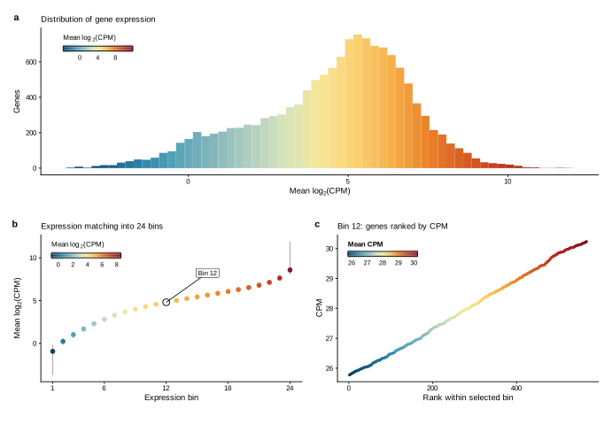
For expression matching, the function averages each gene across the available samples and assigns it to one of nbin bins. Let $M$ be the requested module genes that are present in the matrix. For each gene in $M$, it samples up to ctrl eligible controls from the same expression bin; the unique sampled controls form $C$. Genes requested in any supplied module are excluded from the control universe, and the nearest available bin is used only when an exact bin has no eligible controls.

For one sample, let $x_g$ be the normalized expression of gene $g$. The bulk module score (BMS) is

\[ \operatorname{BMS} = \frac{1}{|M|}\sum_{g \in M} x_g - \frac{1}{|C|}\sum_{g \in C} x_g. \]

Here, $g$ is a gene being summed, $M$ is the set of retained module genes, $C$ is the pooled set of matched controls, and $|M|$ and $|C|$ are their gene counts. The first term is the module’s mean expression; the second is the matched-control mean. Missing requested genes are omitted and recorded in audit.

flowchart TD
    X["Normalized expression matrix<br/>(genes × samples)"] --> B["Average each gene across samples<br/>and assign an expression bin"]
    G["Named gene set"] --> M["Retain genes present in the matrix"]
    B --> C["For each retained gene, sample up to ctrl<br/>eligible non-module genes from its bin"]
    M --> C
    X --> U["Mean retained module-gene expression<br/>within each sample"]
    M --> U
    X --> V["Mean pooled-control expression<br/>within each sample"]
    C --> V
    U --> S["Bulk module score<br/>module mean − control mean"]
    V --> S

Figure 1. Construction of one expression-matched bulk module score. Expression bins define the eligible controls; the two per-sample means are then subtracted.

3 Example dataset

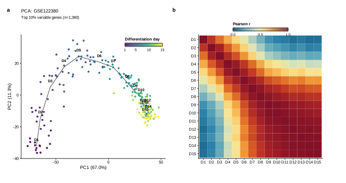
The example uses GSE122380, a bulk RNA-seq time course of induced pluripotent stem cell differentiation toward cardiomyocytes.⁴ The processed data contain 192 samples from 13 cell lines across 15 days. Each cell line contributes at most one library per day.

The scoring matrix contains DESeq2 variance-stabilizing transformation values.³

Table 3.1: GSE122380 tutorial data at a glance.
Samples	Cell lines	Days	Samples per day
192	13	1–15	12–13

Figure 2. Structure of the GSE122380 differentiation time course. a. PCA of all samples using the top 10% most variable VST genes, colored by differentiation day. b. Pearson correlation matrix of day-averaged profiles using the same genes; Pearson correlation is a descriptive similarity measure.

4 Calculation

The expression-bin diagnostic below uses the supplied log2 CPM matrix. It shows the full expression distribution, the range and median of each bin, and the genes in one representative bin.

Figure 3. Expression-bin matching. a. Distribution of average log2 CPM across genes. b. Median and range for each of 24 expression bins; the outlined point marks bin 12. c. Genes within bin 12 ordered by average CPM.

calc_bulk_module_score() returns a bulk_module_score_result with:

scores: one row per sample and one score column per module;
audit: requested, present, missing, and pooled-control counts by module_id;
genes: requested, present, and missing identifiers;
controls: per-gene and pooled control identifiers; and
params: effective binning, control, seed, and control-universe settings.

The worked examples below show the data preview, scoring call, and returned data. The same matrix, ordered gene-set list, arguments, and seed reproduce the same controls and scores without changing the caller’s random-number state. Scores are relative to the matched background in the analyzed matrix; they are not absolute pathway-activity measurements.

5 Why matched controls?

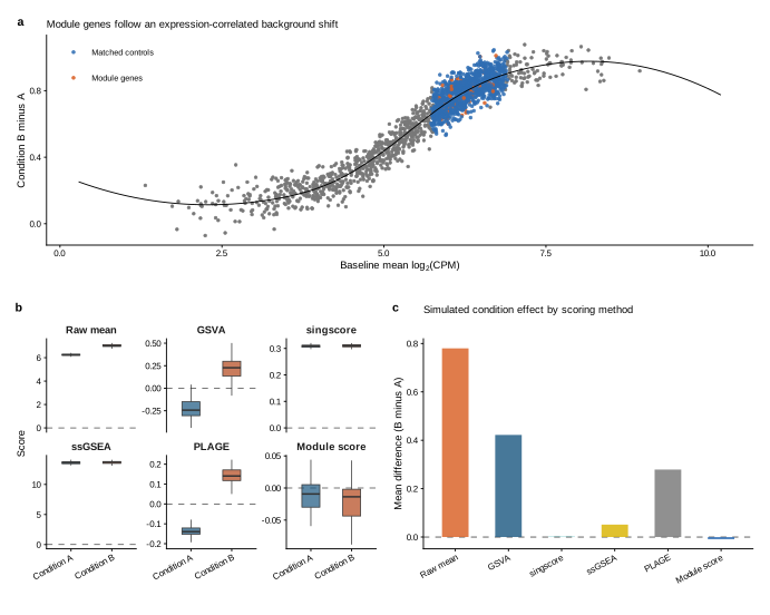
Average gene expression can track broad technical or biological background shifts. The simulation below gives high-expression module genes a condition-associated shift but no module-specific effect, then compares six single-sample summaries. It illustrates the purpose of expression matching rather than benchmarking the methods across datasets.

Figure 4. Simulated expression-correlated background change. a. Module genes and matched controls occupy similar expression ranges and share a background shift. b. Sample scores by condition for six summaries; dashed lines mark zero. c. Mean condition difference for each summary, using the same categorical palette as the other tutorial figures.

6 Worked examples

6.1 Public gene sets

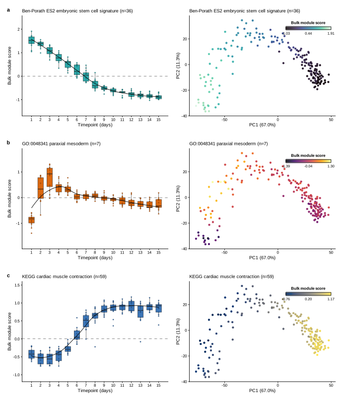
The runner uses three memberships pinned in data/GSE122380_public_gene_sets.csv: Ben-Porath ES2, GO:0048341 paraxial mesoderm formation, and the KEGG legacy cardiac muscle contraction set. The file records MSigDB release 2026.1.Hs, so later database updates cannot silently change this analysis.

stem_signature_genes <- head(reference_sets$embryonic_stem_cell_signature, 10L)
vst_matrix[
    stem_signature_genes[stem_signature_genes %in% rownames(vst_matrix)],
    seq_len(5L),
    drop = FALSE
]
#>          18489_10  18489_11  18489_12  18489_13  18489_14
#> AEN     10.019050  9.834333  9.804758 10.120719 10.104353
#> CDC25A   9.190262  9.487755  9.440176  9.680939  9.238891
#> CHEK2    9.118110  8.702930  8.918427  9.152482  9.058191
#> CLDN6   13.192216 13.129604 12.570583 13.011490 12.687951
#> CRIPTO   9.062016  8.993060  8.352598  9.041377  8.557690
#> CYP26A1  7.696863  7.679195  8.120473  7.854711  8.080204
#> DBNDD1   8.253144  8.152396  8.157294  8.205546  8.085414
#> DNMT3A  11.616437 11.565719 11.592819 11.634917 11.413029
#> DSCC1    7.853225  8.206465  8.279924  8.506173  7.909179
#> DTYMK    9.330298  9.536974  9.448221  9.639711  9.420154

The preview shows VST values for the available genes from the embryonic stem-cell signature, with genes in rows and samples in columns.

The full scoring call specifies the control universe and all parameters that affect control selection. scores is the sample-level result; audit verifies the genes retained and controls used for each module.

reference_scores <- calc_bulk_module_score(
    x = vst_matrix,
    gene_sets = reference_sets,
    universe = NULL,
    nbin = 24L,
    ctrl = 100L,
    seed = 1L
)

head(reference_scores$scores, 5L)
#>   sample_id embryonic_stem_cell_signature paraxial_mesoderm
#> 1  18489_10                    -0.6716225        -0.1422926
#> 2  18489_11                    -0.7060135        -0.2521477
#> 3  18489_12                    -0.7801974        -0.3642349
#> 4  18489_13                    -0.6753000        -0.3584454
#> 5  18489_14                    -0.8463461        -0.4639695
#>   kegg_cardiac_muscle_contraction
#> 1                       1.0344600
#> 2                       0.9468760
#> 3                       0.7376880
#> 4                       0.9016347
#> 5                       0.7460066

reference_scores$audit
#>                         module_id n_requested n_present n_missing n_controls
#> 1   embryonic_stem_cell_signature          40        36         4       3197
#> 2               paraxial_mesoderm           7         7         0        700
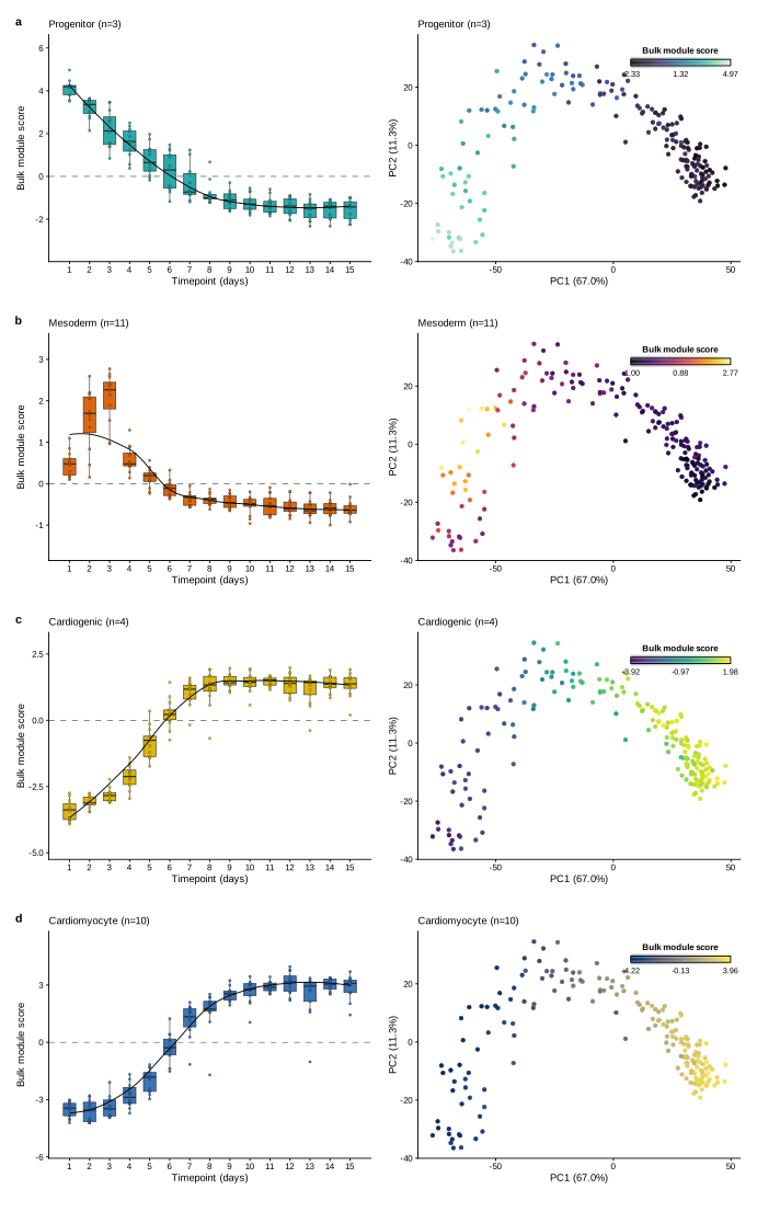
#> 3 kegg_cardiac_muscle_contraction          79        59        20       4224

The boxplots show sample distributions by day, a smooth fit through daily medians, and a dashed zero line. The paired PCA panels color the same samples by score without adding a trajectory path.

Figure 5. Public gene-set module scores across GSE122380. Each row pairs a day-level boxplot with a PCA score overlay. Gene counts reflect identifiers present in the VST matrix.

6.2 Custom marker sets

Custom gene lists use the same interface. These examples follow progenitor, mesoderm, cardiogenic, and cardiomyocyte markers through the differentiation series.

marker_scores <- calc_bulk_module_score(
    x = vst_matrix,
    gene_sets = marker_sets,
    universe = NULL,
    nbin = 24L,
    ctrl = 100L,
    seed = 1L
)

head(marker_scores$scores, 5L)
#>   sample_id progenitor   mesoderm cardiogenic cardiomyocyte
#> 1  18489_10  -1.066637 -0.7898060   1.4361839      3.042434
#> 2  18489_11  -1.110534 -0.8209258   1.4665504      2.966914
#> 3  18489_12  -1.056210 -0.7768030   1.0065031      2.592528
#> 4  18489_13  -1.062145 -0.9443249   1.4240485      2.965420
#> 5  18489_14  -1.204518 -0.7713819   0.8473344      2.557726

marker_scores$audit
#>       module_id n_requested n_present n_missing n_controls
#> 1    progenitor           5         3         2        300
#> 2      mesoderm          11        11         0       1050
#> 3   cardiogenic           4         4         0        400
#> 4 cardiomyocyte          10        10         0        789

The same smooth median summaries are drawn for the custom marker sets; PCA points are colored by score without a connecting trajectory.

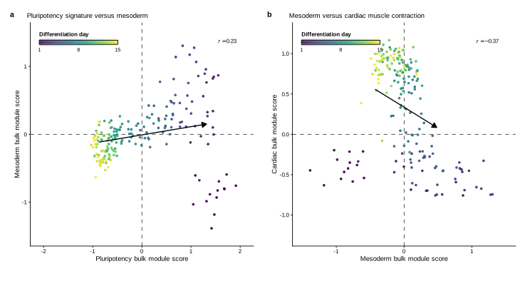
Figure 6. Custom marker-set module scores. Each row pairs the day-level score distribution with a PCA overlay.

The pairwise plots summarize co-variation among public module scores. Each panel centers both axes on zero and includes its own differentiation-day legend. Arrows follow fitted linear trends from the lower to the upper decile of each x-axis score. Pearson’s $r$ is descriptive because the scores and differentiation days are structured; it is not a causal model or an independent-sample significance test.

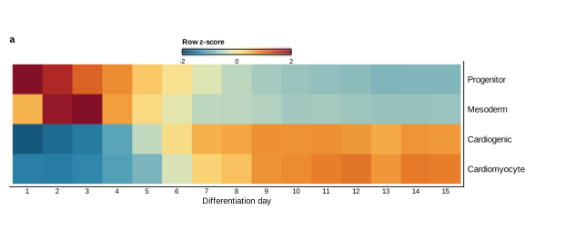
Figure 7. Relationships among public module scores. Color indicates differentiation day; each scatterplot has its own legend in the upper-left corner. Dashed axes mark zero, and arrows show fitted trend direction. Pearson’s r is descriptive.

The heatmap averages scores within each day and standardizes each marker-set trajectory to a row z-score, emphasizing temporal shape rather than absolute magnitude.

Figure 8. Day-averaged custom marker-set scores standardized within each row.

7 Matched-bin permutation analysis

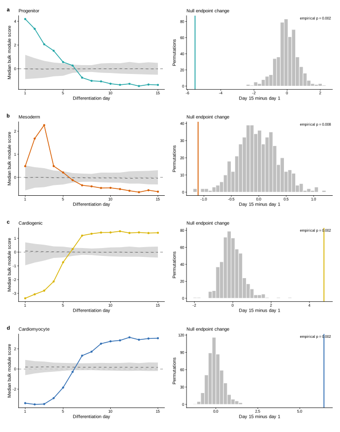
perm_bulk_module_score() compares one observed gene set with null sets of the same size. null_method = 'matched_bins' preserves the observed set’s expression-bin composition. This analysis summarizes each day by its median score and compares the day 15 minus day 1 change with the null distribution.

Values in group_col must be complete for all matrix samples. Factor levels define the endpoint order; non-factor values are sorted. The resolved order is returned in params$group_levels.

permutation_result <- perm_bulk_module_score(
    x = vst_matrix,
    gene_set = marker_sets$cardiomyocyte,
    metadata = GSE122380_metadata,
    group_col = 'day',
    n_perm = 500L,
    null_method = 'matched_bins',
    universe = NULL,
    nbin = 24L,
    ctrl = 100L,
    seed = 104L,
    group_summary = 'median',
    trajectory_statistic = 'last_minus_first',
    alternative = 'two.sided'
)

trajectory reports the observed endpoint change and its matched-bin null distribution. group_summary reports the observed median score, null interval, and empirical p-value at each day.

permutation_result$trajectory
#>          statistic observed   null_mean   null_sd empirical_p
#> 1 last_minus_first 6.440761 -0.01508637 0.4476247 0.001996008
permutation_result$group_summary
#>    group observed_score null_mean null_median   null_sd null_lower null_upper
#> 1      1     -3.3902715 0.1849032   0.1937655 0.3676797 -0.6130279  0.9012390
#> 2      2     -3.5129926 0.1937007   0.1863426 0.3094676 -0.4439280  0.7754273
#> 3      3     -3.4798363 0.2002105   0.2076014 0.2673984 -0.3318638  0.7336975
#> 4      4     -2.8954708 0.2041132   0.1997583 0.2167013 -0.2662862  0.6309592
#> 5      5     -1.8422259 0.2037541   0.2005287 0.2066237 -0.1855468  0.6028672
#> 6      6     -0.2863119 0.1939426   0.1825010 0.1833552 -0.1250247  0.5828230
#> 7      7      1.3196850 0.1840214   0.1661723 0.1782938 -0.1219788  0.5667898
#> 8      8      1.7128665 0.1815939   0.1707553 0.1792685 -0.1127352  0.5797209
#> 9      9      2.5076165 0.1749028   0.1718002 0.1909906 -0.1498529  0.6033562
#> 10    10      2.7390175 0.1737691   0.1602729 0.1978658 -0.1641389  0.5885609
#> 11    11      2.8327956 0.1715812   0.1707253 0.1984719 -0.1875231  0.5949097
#> 12    12      3.1339879 0.1697262   0.1653626 0.2106911 -0.1929123  0.6334362
#> 13    13      2.8996045 0.1732159   0.1588241 0.2005042 -0.1784600  0.5813966
#> 14    14      3.0172505 0.1681251   0.1592695 0.2093395 -0.2012848  0.6480631
#> 15    15      3.0504899 0.1698168   0.1575988 0.2125369 -0.2001207  0.6370908
#>    empirical_p
#> 1  0.001996008
#> 2  0.001996008
#> 3  0.001996008
#> 4  0.001996008
#> 5  0.001996008
#> 6  0.015968064
#> 7  0.001996008
#> 8  0.001996008
#> 9  0.001996008
#> 10 0.001996008
#> 11 0.001996008
#> 12 0.001996008
#> 13 0.001996008
#> 14 0.001996008
#> 15 0.001996008

7.0.1 Empirical p-value

For n_perm null sets, the empirical p-value is

\[ p = \frac{b + 1}{n_{perm} + 1}, \]

where $b$ is the number of null statistics at least as extreme as the observed statistic under the selected alternative. With 500 permutations, the smallest attainable p-value is $1 / 501$. This is a gene-set null test, not a sample-level model of the experimental design.

Figure 9. Matched-bin permutation diagnostics for custom marker sets. Left panels compare observed median trajectories with the median and 95% interval of null trajectories. Right panels show null endpoint-change distributions; colored lines mark observed changes.

8 Interpretation and limitations

Normalize and filter the expression matrix before scoring, and use one identifier convention for matrix rows and gene sets.
Inspect audit and genes; absent module genes are omitted rather than imputed.
Record the ordered gene sets, control universe, nbin, ctrl, and seed because together they define control selection.
Compare scores within a consistently processed matrix. Independently processed datasets can have different matched backgrounds.
Treat the correlation, trajectory, and permutation summaries according to their stated descriptive or gene-set-null roles.

9 Session information

sessionInfo()
#> R version 4.6.1 (2026-06-24)
#> Platform: aarch64-apple-darwin23
#> Running under: macOS Tahoe 26.5.1
#> 
#> Matrix products: default
#> BLAS:   /Library/Frameworks/R.framework/Versions/4.6/Resources/lib/libRblas.0.dylib 
#> LAPACK: /Library/Frameworks/R.framework/Versions/4.6/Resources/lib/libRlapack.dylib;  LAPACK version 3.12.1
#> 
#> locale:
#> [1] C.UTF-8/C.UTF-8/C.UTF-8/C/C.UTF-8/C.UTF-8
#> 
#> time zone: America/New_York
#> tzcode source: internal
#> 
#> attached base packages:
#> [1] stats     graphics  grDevices utils     datasets  methods   base     
#> 
#> other attached packages:
#> [1] magrittr_2.0.5
#> 
#> loaded via a namespace (and not attached):
#>  [1] crayon_1.5.3      vctrs_0.7.3       cli_3.6.6         knitr_1.51       
#>  [5] rlang_1.3.0       xfun_0.60         otel_0.2.0        generics_0.1.4   
#>  [9] jsonlite_2.0.0    bit_4.6.0         glue_1.8.1        htmltools_0.5.9  
#> [13] sass_0.4.10       hms_1.1.4         rmarkdown_2.31    evaluate_1.0.5   
#> [17] jquerylib_0.1.4   tibble_3.3.1      tzdb_0.5.0        fastmap_1.2.0    
#> [21] yaml_2.3.12       lifecycle_1.0.5   bookdown_0.47     compiler_4.6.1   
#> [25] dplyr_1.2.1       pkgconfig_2.0.3   rstudioapi_0.19.0 digest_0.6.39    
#> [29] R6_2.6.1          tidyselect_1.2.1  readr_2.2.0       parallel_4.6.1   
#> [33] vroom_1.7.1       pillar_1.11.1     bslib_0.11.0      bit64_4.8.2      
#> [37] tools_4.6.1       withr_3.0.3       cachem_1.1.0

References

1. Satija Lab. AddModuleScore reference and source code.

2. Tirosh I, Izar B, Prakadan SM, et al. Dissecting the multicellular ecosystem of metastatic melanoma by single-cell RNA-seq. Science. 2016;352(6282):189-196.

3. Love MI, Huber W, Anders S. Moderated estimation of fold change and dispersion for RNA-seq data with DESeq2. Genome Biology. 2014;15:550.

4. Strober BJ, Elorbany R, Rhodes K, et al. Dynamic genetic regulation of gene expression during cellular differentiation. Science. 2019;364(6447):1287-1290. Dataset: GSE122380.

Expression-matched bulk scoring