Gene set enrichment analysis NES waterfall, volcano, and comparative scatter plots
Gene set enrichment analysis NES waterfall, volcano, and comparative scatter plots
1 Overview
This repository contains several functions that generate useful visualizations of precomputed Gene Set Enrichment Analysis (GSEA) results. These visualizations include (1) ranked (by NES) waterfall plots with biological categorizations, (2) NES volcano plots for a specific DEG contrast, and cross-contrast comparative NES scatterplots.
Note that the functions demonstrated in this workflow assume GSEA has been performed on your
DEG contrast of interest. Therefore, I recommended generating the required GSEA results data
using one of the many options available via Bioconductor, such as fgsea or clusterProfiler.
1.1 Issues with GSEA dotplots/barplots
GSEA results are most commonly visualized as running enrichment score plots for an individual GO/KEGG/Reactome pathway result, or as dotplot/barplot-style summaries of a short list of terms in which dot size or color indicates some quantitative GSEA metric (NES or adjusted p-value, for example). Those GSEA visualizations typically shown for the top ~n=10 enriched GO terms (by NES) due to space constraints with a greater number of pathways. Therefore the broader ranked GSEA results are often lost if only the top 10 pathways are shown. For example, if there are 200 total significantly enriched GO terms (by adjusted p-value < 0.05) and only the top 10 GO terms (by +NES) are visualized, then 190/200 = 95% of total enriched terms are not shown. This loss of information can be particularly problematic if, for example, the top 10 enriched GO terms by GSEA NES are concentrated in the same biological function or some particular pathway, which can often be the case for more general, larger GO term families (e.g: cell cycle replication, extracellular matrix, etc).
1.2 Use case
The ranked GSEA waterfall plots shown in the tutorial workflow are intended to address the limitation of the aformentioned GSEA dotplot/barplot. Ranked GSEA waterfall plots allow for visualization from 50–200 ranked GO terms one concise, visually cohesive, and customizable figure panel. The GSEA-derived metric used to rank GO terms for the waterfall plot can be selected by the user; though I recommend use NES, as this makes comparisons between the magnitude of enrichment between GO terms containing differing numbers of genes (and effect size is a more biologically informative metric than statistical significance for GSEA).
Because it would be impractical to write out the GO term labels for all 100 pathways (not enough
space in a single figure panel for this. Even if it were possible to do this, it would be visually
incoherent), user-defined color_by_groups are used to organize the top n=X ranked GO terms by
biological theme/functional process. Note that these classifications
For the waterfall plots, the user can select specific colors to define these biological groupins.
In the example workflow, for example, I categorized GO term pathways by Ion channel,
Metabolism, Muscle contraction, Heart development, and Other. Here, Other simply means .
I want to note that these categorizations/classifications are simply user-defined annotations only and do not perform redundancy reduction. For example, for the positive NES waterfall plot,
'Metabolism' = c('mitochondrial', 'metabolic', 'oxidative')
The visual design was informed by figures shown in Ciceri et al. (2024), Xu et al. (2025), Vuong et al. (2026), and Risgaard et al. (2026). In particular, see the following subpanels from Xu et al. Figure 3X; from Vuong et al. Figure 3X; from Ciceri et al. Figure 3X; from Risgaard et al. Figure 3X. Full citations are provided at the end of this README.
1.3 Example data used in workflow/tutorial
The bundled tables used for the figures generated in the workflow/tutorial are derived from the public NCBI GEO accession GSE122380, a bulk RNA-seq time course of human iPSC differentiation into cardiomyocytes. Basic sequencing and sample-level QC was performed before differential expression analysis. A DESeq2 comparison of day 9 (cardiomyocyte) versus day 3 (mesoderm) generated the cardiomyocyte-versus-mesoderm contrast used for the bundled GSEA results.
2 Install and source
To download the R scripts containing the functions used to generate the GSEA results visualizations, run the following line of code below in your R console. The below command will download the R script to your present working directory.
download.file(
  'https://raw.githubusercontent.com/ZohebKhan1/gsea-waterfall/main/functions/gsea_visualizations.R',
  'gsea_visualizations.R'
)
In the relevant R script, source the downloaded R script, assuming it is in your project root
directory. gsea_visualizations.R contains the following functions: read_gsea_result_csv(),
plot_gsea_waterfall(), plot_gsea_volcano(), plot_gsea_half_volcano(), and
plot_gsea_nes_scatter(). The visualizations generated by these functions can be seen in the
published GitHub Pages site linked at the start of this README.md.
3 Required input GSEA data format
For all GSEA visualizations in this repository, the input dataframe represents one GSEA contrast with one row per unique term:
The completed result table can come from any GSEA workflow, including fgsea,
clusterProfiler, or another package. If the source uses different column
names, map them when reading the table as shown below.
| Column | Required | Meaning |
|---|---|---|
go_description |
yes | term description and fallback matching key |
go_term_id |
no | stable matching key used automatically when present |
NES |
yes | normalized enrichment score |
pval |
no | optional nominal GSEA p-value; used only for nominal-p-value ranking or y-axes |
padj |
yes | adjusted p-value in [0, 1] |
go_description, NES, and padj must be complete; NES values must be finite.
If pval is supplied, it is also validated. Key precedence is explicit
id_col, then go_term_id when present, otherwise go_description.
Comparative plots use the exact shared-key intersection and do not impute absent
terms.
fgsea_results <- read_gsea_result_csv(
  'fgsea_results.csv',  # unformatted GSEA results .csv file
  term_col = 'pathway', # column name for GO term description
  nes_col = 'NES',      # column name for normalized enrichment score
  padj_col = 'padj'     # column name for adjusted p-value (for filtering)
)
Load the bundled examples:
source('../functions/gsea_visualizations.R')

gsea_cardiomyocyte_vs_mesoderm <- read_gsea_result_csv(
  'data/GSE122380_gsea_cardiomyocyte_vs_mesoderm.csv'
)

gsea_day9_vs_day6 <- read_gsea_result_csv(
  'data/GSE122380_gsea_day9_vs_day6.csv'
)

gsea_day3_vs_day1 <- read_gsea_result_csv(
  'data/GSE122380_gsea_day3_vs_day1.csv'
)

print(head(gsea_cardiomyocyte_vs_mesoderm, 5L))
## go_term_id go_description NES
## 1 DNA replication DNA replication -3.251308
## 2 chromosome segregation chromosome segregation -2.816035
## 3 DNA-templated DNA replication DNA-templated DNA replication -3.335061
## 4 ribosome biogenesis ribosome biogenesis -2.989959
## 5 cell cycle checkpoint signaling cell cycle checkpoint signaling -3.032195
## pvalue padj pval
## 1 2.397081e-45 5.949555e-42 2.397081e-45
## 2 9.005650e-36 1.117601e-32 9.005650e-36
## 3 4.266279e-35 3.529635e-32 4.266279e-35
## 4 1.159752e-34 7.196264e-32 1.159752e-34
## 5 1.003151e-28 4.149703e-26 1.003151e-284 Ranked GSEA waterfall plots
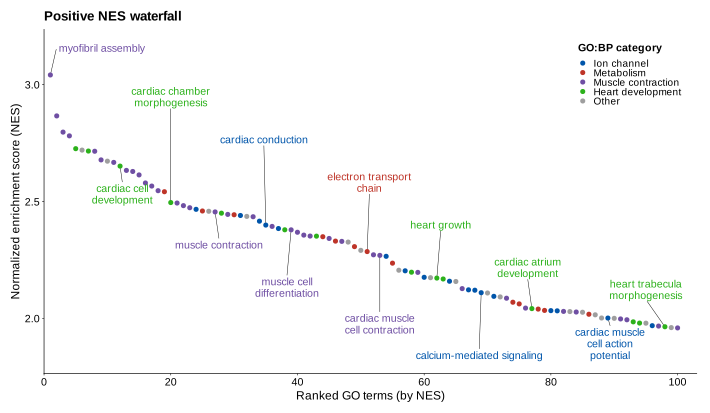
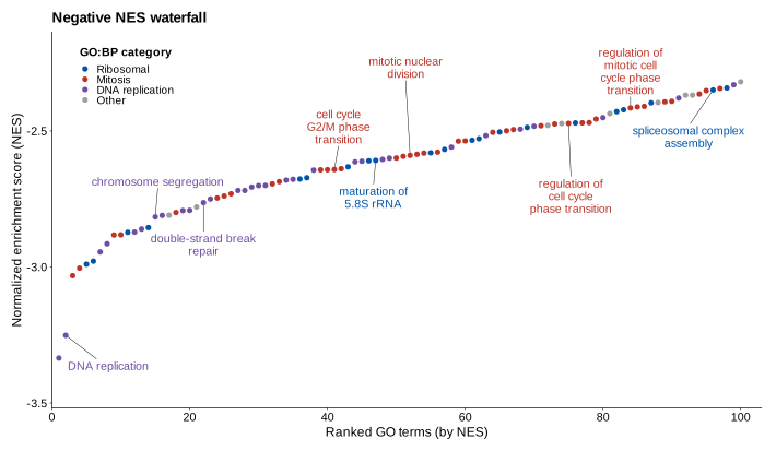
plot_gsea_waterfall() first applies the optional padj_threshold, selects one NES direction,
ranks by NES or padj by default, and retains top_n terms. Nominal-p-value ranking is
available when an optional pval column is supplied. color_by_groups controls colors and
label_by_groups controls labels. Matches are case-insensitive against term descriptions or IDs.
For the example waterfall figures, classifications use caller-defined keyword
groups for ion-channel, metabolic, muscle-contraction, heart-development,
ribosomal, mitotic, and DNA-replication terms; unmatched terms remain Other.
4.1 Positive NES waterfall
# Read and format the GSEA results.
gsea_cardiomyocyte_vs_mesoderm <- read_gsea_result_csv(
  'tutorial/data/GSE122380_gsea_cardiomyocyte_vs_mesoderm.csv'
)

# Choose GO terms to label with text on the GSEA waterfall plot.
positive_waterfall_label_terms <- c(
  'myofibril assembly',
  'cardiac muscle cell action potential',
  'calcium-mediated signaling',
  'electron transport chain',
  'muscle cell differentiation',
  'cardiac cell development',
  'cardiac chamber morphogenesis',
  'muscle contraction',
  'cardiac conduction',
  'cardiac muscle cell contraction',
  'heart growth',
  'cardiac atrium development',
  'heart trabecula morphogenesis'
)

# Choose words used to color GO terms by biological category.
color_by_group_categories <- list(
  'Ion channel' = c(
    'Calcium', 'Sodium', 'Potassium', 'Ion', 'Voltage', 'Channel',
    'electrical', 'Action potential', 'transmembrane', 'conduction'
  ),
  'Metabolism' = c(
    'Metabolic', 'Metabolism', 'Electron transport chain', 'Mitochondria',
    'Mitochondrial', 'Oxidative', 'Phosphorylation', 'ATP', 'lipid',
    'biosynthetic', 'respiration'
  ),
  'Muscle contraction' = c(
    'Muscle contraction', 'Muscle cell differentiation', 'Striated',
    'Sarcomere', 'Myofibril', 'Actin', 'Muscle'
  ),
  'Heart development' = c(
    'atrial', 'ventricular', 'heart', 'cardiac'
  )
)

# Create the positive-NES GSEA waterfall plot.
positive_waterfall_plot <- plot_gsea_waterfall(
  gsea_results = gsea_cardiomyocyte_vs_mesoderm, # formatted GSEA results
  padj_threshold = 0.05, # adjusted p-value cutoff for significant GO terms
  NES_direction = 'positive', # plot GO terms with positive NES values
  top_n = 100, # total number of GO terms to rank and plot
  rank_by = 'NES', # metric used to rank the GO terms
  label_by_groups = positive_waterfall_label_terms, # character vector of GO terms to label
  color_by_groups = color_by_group_categories # named list of biological categories and matching words
)
padj_threshold = 0.05 retains only terms with adjusted p-value below 0.05 before ranking.
NES_direction then chooses the NES side to display, and top_n is applied after filtering and
ranking. Terms are neutral unless color_by_groups is supplied; each seed is matched
case-insensitively against term IDs or descriptions.
4.2 Negative NES waterfall
# Read and format the GSEA results.
gsea_cardiomyocyte_vs_mesoderm <- read_gsea_result_csv(
  'tutorial/data/GSE122380_gsea_cardiomyocyte_vs_mesoderm.csv'
)

# Choose GO terms to label with text on the GSEA waterfall plot.
negative_waterfall_label_terms <- c(
  'DNA replication',
  'chromosome segregation',
  'double-strand break repair',
  'cell cycle G2/M phase transition',
  'maturation of 5.8S rRNA',
  'mitotic nuclear division',
  'regulation of cell cycle phase transition',
  'regulation of mitotic cell cycle phase transition',
  'spliceosomal complex assembly'
)

# Choose words used to color GO terms by biological category.
negative_color_by_group_categories <- list(
  'Ribosomal' = c(
    'ribosome', 'ribosomal', 'spliceosomal', 'rRNA', 'RNA'
  ),
  'Mitosis' = c(
    'Mitosis', 'Meiosis', 'Nuclear division', 'cell cycle', 'telomere',
    'spindle', 'Mitotic', 'Meiotic'
  ),
  'DNA replication' = c(
    'chromosome', 'DNA', 'base', 'repair', 'DNA-'
  )
)

# Create the negative-NES GSEA waterfall plot.
negative_waterfall_plot <- plot_gsea_waterfall(
  gsea_results = gsea_cardiomyocyte_vs_mesoderm, # formatted GSEA results
  padj_threshold = 0.05, # adjusted p-value cutoff for significant GO terms
  NES_direction = 'negative', # plot GO terms with negative NES values
  top_n = 100, # total number of GO terms to rank and plot
  rank_by = 'NES', # metric used to rank the GO terms
  label_by_groups = negative_waterfall_label_terms, # character vector of GO terms to label
  color_by_groups = negative_color_by_group_categories # named list of biological categories and matching words
)
Use rank_by = 'padj' when adjusted-p-value ranking, rather than NES magnitude,
should determine the displayed order. rank_by = 'pvalue' is available when an
optional nominal pval column is supplied. label_n selects labels
automatically when exact terms are not supplied; use label_by_groups when
specific terms should be shown.
5 Volcano plots
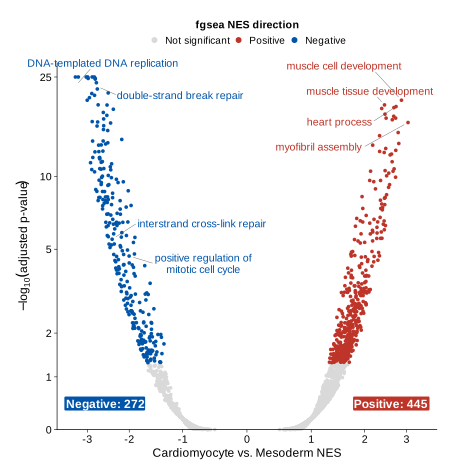
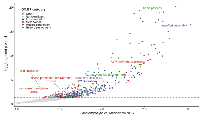
Use plot_gsea_volcano() for both NES directions in one panel and plot_gsea_half_volcano() for
a directional view. These plots retain significant and nonsignificant GO terms. The
padj_cutoff = 0.05 setting controls significance coloring without filtering rows.
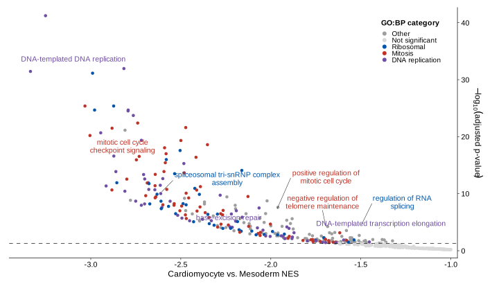
5.1 Symmetric volcano
The example labels four padj-significant terms across each NES direction, from
approximately NES 2 to the most extreme observed value. The same terms are
used in the symmetric volcano. Directional half-volcano labels are selected
separately from significant terms assigned to caller-defined groups; Other
and Not significant terms are not labeled.
negative_volcano_label_terms <- c(
  'DNA-templated DNA replication',
  'double-strand break repair',
  'interstrand cross-link repair',
  'positive regulation of mitotic cell cycle'
)

positive_volcano_label_terms <- c(
  'muscle tissue development',
  'heart process',
  'muscle cell development',
  'myofibril assembly'
)

volcano_label_terms <- c(
  negative_volcano_label_terms,
  positive_volcano_label_terms
)

positive_half_volcano_label_terms <- c(
  'response to oxidative stress',
  'lipid localization',
  'ribose phosphate biosynthetic process',
  'smooth muscle cell proliferation',
  'cardiac ventricle development',
  'ATP biosynthetic process',
  'heart process',
  'myofibril assembly'
)

negative_half_volcano_label_terms <- c(
  'DNA-templated DNA replication',
  'mitotic cell cycle checkpoint signaling',
  'spliceosomal tri-snRNP complex assembly',
  'base-excision repair',
  'positive regulation of mitotic cell cycle',
  'negative regulation of telomere maintenance',
  'regulation of RNA splicing',
  'DNA-templated transcription elongation'
)
symmetric_volcano_plot <- plot_gsea_volcano(
gsea_results = gsea_cardiomyocyte_vs_mesoderm,
padj_cutoff = 0.05,
label_terms = volcano_label_terms,
contrast_label = 'Cardiomyocyte vs. Mesoderm',
label_words_per_line = 3L,
point_size = 1.30
)padj_cutoff controls significance coloring and the displayed counts without removing terms.
Nonsignificant GO terms remain visible in grey. Use label_terms instead of label_n when you
want to label exact terms.
5.2 Directional half-volcano plots
positive_half_volcano_plot <- plot_gsea_half_volcano(
  gsea_results = gsea_cardiomyocyte_vs_mesoderm,
  direction = 'positive',
  p_col = 'padj',
  padj_cutoff = 0.05,
  label_terms = positive_half_volcano_label_terms,
  term_groups = color_by_group_categories,
  inner_nes_limit = 1,
  contrast_label = 'Cardiomyocyte vs. Mesoderm',
  point_size = 1.60
)
inner_nes_limit = 1 keeps terms with positive NES at least 1 in magnitude.
Set p_col = 'pvalue' to show nominal p-values when the optional pval column
is supplied; significance coloring continues to use padj_cutoff.
negative_half_volcano_plot <- plot_gsea_half_volcano(
  gsea_results = gsea_cardiomyocyte_vs_mesoderm,
  direction = 'negative',
  p_col = 'padj',
  padj_cutoff = 0.05,
  label_terms = negative_half_volcano_label_terms,
  term_groups = negative_color_by_group_categories,
  inner_nes_limit = 1,
  contrast_label = 'Cardiomyocyte vs. Mesoderm',
  point_size = 1.60
)
6 Comparative NES scatterplot
plot_gsea_nes_scatter() compares exact shared term keys and retains significant
and nonsignificant terms by default. Nonsignificant terms are shown in grey. The
optional fitted line is descriptive and does not alter enrichment statistics.
nes_scatter_label_terms <- c(
  'mesenchyme development',
  'mesoderm development',
  'mesodermal cell differentiation',
  'myofibril assembly',
  'heart process',
  'oxidative phosphorylation',
  'regulation of nuclear division'
)

nes_scatter_plot <- plot_gsea_nes_scatter(
  gsea_x = gsea_day9_vs_day6,
  gsea_y = gsea_day3_vs_day1,
  x_label = 'Day 9 vs. Day 6 NES',
  y_label = 'Day 3 vs. Day 1 NES',
  color_by = 'significance',
  quadrant = 'all',
  x_name = 'Day 9 vs. Day 6',
  y_name = 'Day 3 vs. Day 1',
  label_terms = nes_scatter_label_terms,
  padj_cutoff = 0.05,
  equal_axis_limits = TRUE,
  show_fit_line = TRUE,
  point_size = 1.30
)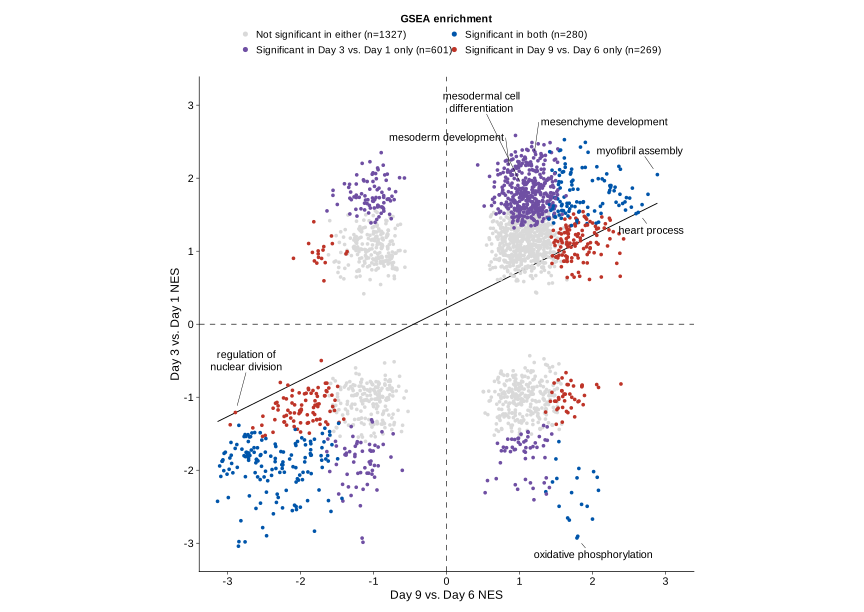
Use quadrant = 'q1' or quadrant = 'q3' to focus on concordant positive or
negative NES values. equal_axis_limits = TRUE makes the two NES axes directly
comparable, while padj_cutoff = 0.05 assigns the significance groups without
removing nonsignificant shared terms.
7 API summary
| Function | Contract |
|---|---|
read_gsea_result_csv() |
reads and validates one precomputed CSV without filtering rows |
plot_gsea_waterfall() |
returns a filtered, ranked one-direction ggplot |
plot_gsea_volcano() |
retains all terms in a symmetric NES-versus-adjusted-p-value ggplot |
plot_gsea_half_volcano() |
retains significant and nonsignificant terms after the directional NES boundary |
plot_gsea_nes_scatter() |
retains the exact shared term-key intersection, including nonsignificant terms |
Source documentation defines the complete argument contracts, including term_col, nes_col,
padj_col, and optional id_col arguments. padj_threshold is specific to the waterfall plot;
nominal-p-value mapping is only needed when using the optional pval-based controls.
8 References
- Subramanian A, Tamayo P, Mootha VK, et al. Gene set enrichment analysis: a knowledge-based approach for interpreting genome-wide expression profiles. PNAS. 2005. https://www.pnas.org/doi/10.1073/pnas.0506580102
- Strober BJ, Elorbany R, Rhodes K, Krishnan N, Tayeb K, Battle A, Gilad Y. Dynamic genetic regulation of gene expression during cellular differentiation. Science. 2019;364(6447):1287-1290. https://doi.org/10.1126/science.aaw0040. Data: NCBI GEO GSE122380.
- Ciceri G, Baggiolini A, Cho HS, et al. An epigenetic barrier sets the timing of human neuronal maturation. Nature. 2024;626:881-890. https://doi.org/10.1038/s41586-023-06984-8
- Xu N, Cho HS, Hackland JOS, et al. Genome-wide CRISPR screen identifies Menin and SUZ12 as regulators of human developmental timing. Nature Cell Biology. 2025;27:1411-1421. https://doi.org/10.1038/s41556-025-01751-5
- Vuong CK, Weber A, Seong P, et al. A single-cell multiomic analysis identifies molecular and gene-regulatory mechanisms dysregulated in developing Down syndrome neocortex. Science. 2026;392:eaea1259. https://doi.org/10.1126/science.aea1259
- Risgaard RD, et al. Molecular and cellular processes disrupted in the early postnatal Down syndrome prefrontal cortex. Science. 2026;392:eaea1549. https://doi.org/10.1126/science.aea1549