Differentiation timing score

Differentiation timing score

PCA-based scoring of differentiation timing from bulk RNA-seq time-course data

Author: Zoheb Khan

Created: 2025-08-29

Modified: 2026-08-10

Compiled: 2026-08-10

Environment: R 4.6.1; Bioconductor 3.23

Dependencies: AnnotationDbi 1.74.0; bookdown 0.47; circlize 0.4.18; clusterProfiler 4.20.0; ComplexHeatmap 2.28.0; DESeq2 1.52.0; edgeR 4.10.1; ggplot2 4.0.3; ggrepel 0.9.8; knitr 1.51; org.Hs.eg.db 3.23.1; patchwork 1.3.2; ragg 1.5.2; scales 1.4.0; systemfonts 1.3.2; viridis 0.6.5

Source: github.com/ZohebKhan1/pca-maturation-scoring

1 Introduction

Bulk RNA-seq differentiation studies usually record samples at discrete timepoints. Samples collected on the same day can still be at different stages of differentiation. This tutorial shows how to use an ordered reference time course to estimate a continuous position for each sample.

The workflow has three stages:

1. Select genes whose expression changes across the reference time course.
2. Fit a PCA space to the reference timepoint means and connect those means into a trajectory.
3. Project each sample onto the trajectory.

The workflow returns a predicted time on the reference scale, a differentiation score scaled from 0 to 1 between the reference endpoints, and squared distance from the trajectory. These outputs describe position within the selected reference; they are not measurements of absolute biological age.

2 Function inputs

get_temporal_genes() uses integer-like raw counts, VST expression, and sample metadata. It selects genes inside the reference cohort. score_differentiation_timing() uses normalized expression and those selected genes to fit the reference PCA and trajectory.

For a reference-only analysis, the scorer uses all supplied samples as the reference. To score new samples, pass reference_samples so that PCA and the trajectory use only the independent reference cohort. Reference samples must have finite timepoints. New non-reference samples can have missing timepoints because the scorer predicts their time rather than using an observed time.

The scorer fits PCA to timepoint means, centers genes, and does not scale them to unit variance. It retains the smallest number of PCs that explain at least 99% of the variance between reference timepoint means. The PCA sign is arbitrary; reversing a PC for a figure does not change distances or scores.

download.file(
  'https://raw.githubusercontent.com/ZohebKhan1/pca-maturation-scoring/main/functions/get_temporal_genes.R',
  'get_temporal_genes.R',
  mode = 'wb'
)
download.file(
  'https://raw.githubusercontent.com/ZohebKhan1/pca-maturation-scoring/main/functions/score_differentiation_timing.R',
  'score_differentiation_timing.R',
  mode = 'wb'
)

source('get_temporal_genes.R')
source('score_differentiation_timing.R')

3 Reference dataset

The example uses processed data from NCBI GEO accession GSE122380, a bulk RNA-seq time course of human induced pluripotent stem cell differentiation into cardiomyocytes. The reference contains 192 samples from 13 cell lines collected across differentiation days 1 through 15.

The repository includes aligned metadata, a raw gene-count matrix, and a VST expression matrix. The tutorial starts from these processed objects. It does not reconstruct the upstream FASTQ processing, read alignment, gene quantification, or VST transformation.

Table 3.1: Samples and represented cell lines by differentiation day.

Metric	D1	D2	D3	D4	D5	D6	D7	D8	D9	D10	D11	D12	D13	D14	D15
Samples	13	12	12	12	13	13	13	13	13	13	13	13	13	13	13
Cell lines	13	12	12	12	13	13	13	13	13	13	13	13	13	13	13

Figure 1 shows the time-course structure with a PCA of the most variable VST genes and a correlation matrix of day-mean expression profiles. Both views show whether the reference has an ordered expression pattern before the trajectory model is fitted.

Figure 1. GSE122380 reference time course and day-level expression correlation. a. PCA using the top 10% most variable VST genes, colored by differentiation day. b. Pearson correlation between day-mean profiles from the same variable-gene set.

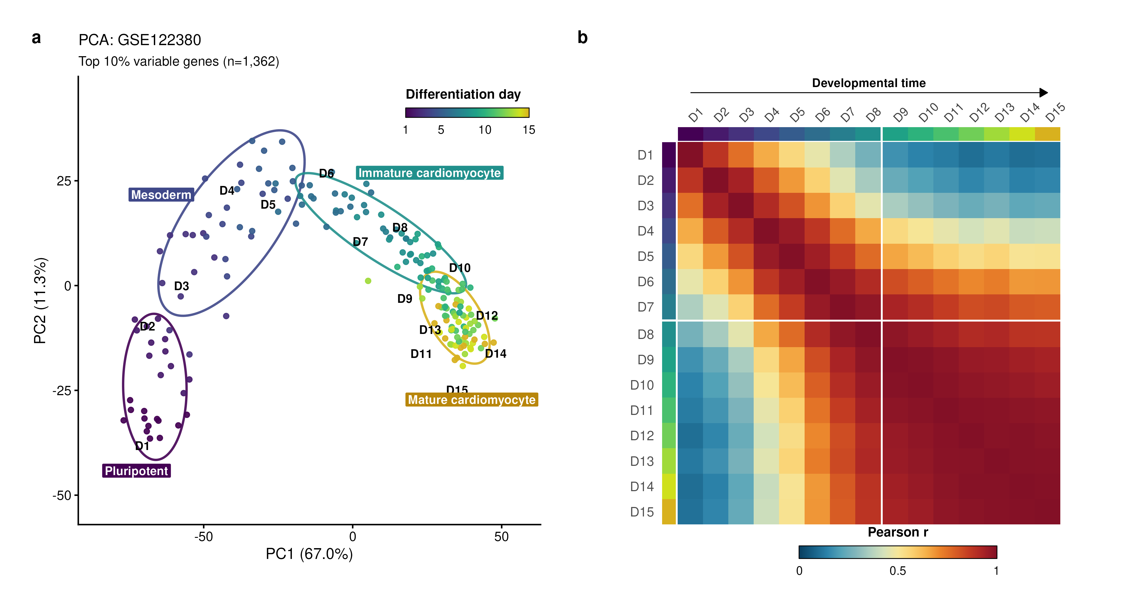
The day ordering is consistent with a reference trajectory. The overview PCA is separate from the scoring PCA, which uses the selected temporal genes and reference timepoint means.

4 Scoring workflow

4.1 Select temporal genes

get_temporal_genes() applies three filters to the reference samples. The function uses raw counts for the expression filter and DESeq2 LRT, and it uses VST expression for the final range filter. A gene must pass every filter to enter the trajectory model.

1. Expression filter. The function calculates TMM-normalized CPM internally. For each gene, it calculates the mean CPM at each reference timepoint and keeps the gene when its largest timepoint mean reaches the expression threshold.
2. DESeq2 likelihood-ratio test. The full model includes categorical time and any requested adjustment covariates. The reduced model contains the adjustment covariates without time. Genes with an adjusted LRT p-value below the selected threshold continue to the final filter.
3. VST-range filter. The function calculates the mean VST expression at each reference timepoint and keeps genes whose range across those means reaches the selected threshold.

The LRT tests whether adding categorical time improves the count model. If the full and reduced models have maximized log likelihoods ell_full and ell_reduced, the likelihood-ratio statistic is

\[ \mathrm{LR} = 2(\ell_\mathrm{full} - \ell_\mathrm{reduced}). \]

The test does not assume that expression changes linearly with time. With no adjustment covariates, the reduced model is ~ 1. For GSE122380, cell_line is included in both models so that the time test accounts for cell-line differences.

source('functions/get_temporal_genes.R')

temporal_selection <- get_temporal_genes(
  raw_counts = counts,
  vst_expression = vst,
  metadata = metadata,
  sample_id_col = 'sample_id',
  time_col = 'day_numeric',
  adjustment_covariates = 'cell_line'
)

temporal_genes <- temporal_selection$temporal_genes

If gene selection should use one reference group, supply reference_group_col and reference_group_value together. The function then restricts the expression filter, LRT, and VST-range filter to samples with that value. This option controls which samples enter selection; it is not a DESeq2 coefficient reference level.

For the GSE122380 reference, the expression, LRT, and VST-range settings produce the counts shown in Table 4.1. For another study, set thresholds from its library sizes, sample size, timepoint coverage, and design.

Table 4.1: Sequential temporal-gene filtering.

Metric	Value
Genes in the aligned count/VST input	13,615
Genes with maximum day-mean TMM CPM >= 10	11,411
Genes passing LRT adjusted p-value < 1e-7	10,863
Genes passing all filters and used for scoring	8,215

The heatmap shows the first 1,500 final temporal genes, ordered by the LRT results. The scoring model uses the complete temporal-gene set, not only the genes shown in this figure.

Figure 2. Heatmap of the 1,500 displayed temporal genes across the reference samples, ordered by differentiation day.

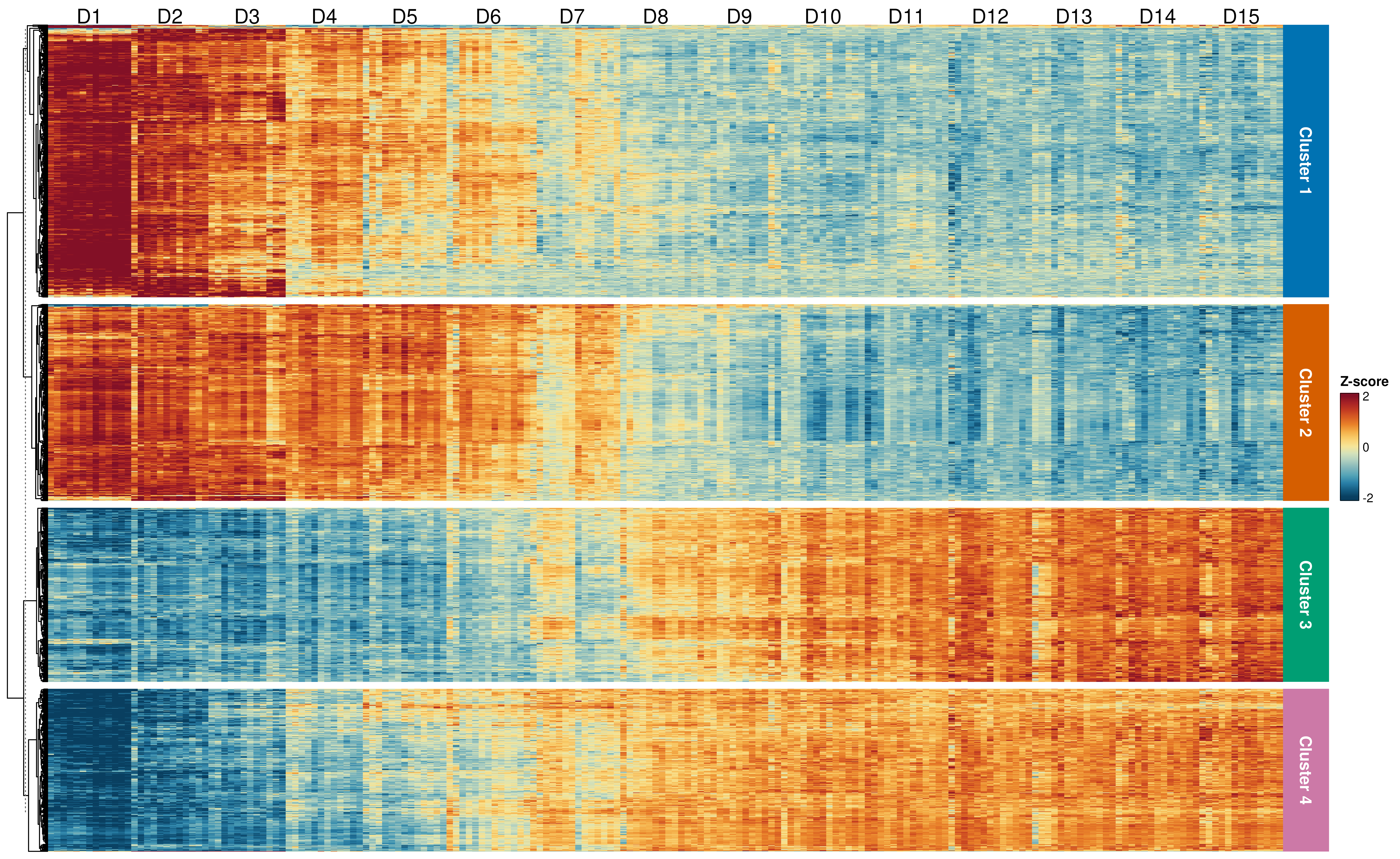
The displayed genes show expression changes across the reference. The display order and heatmap subset are for inspection; PCA, scoring, and validation use all selected temporal genes.

The four clusters in Figure 3 summarize expression patterns in the displayed heatmap genes. They annotate the displayed patterns only. Cluster membership does not change temporal-gene selection, PCA fitting, scoring, or validation. The GO analysis uses the displayed genes as its enrichment universe.

Figure 3. Temporal clusters and GO enrichment for the 1,500 heatmap genes. Each row pairs a cluster trajectory with its top enriched GO Biological Process terms.

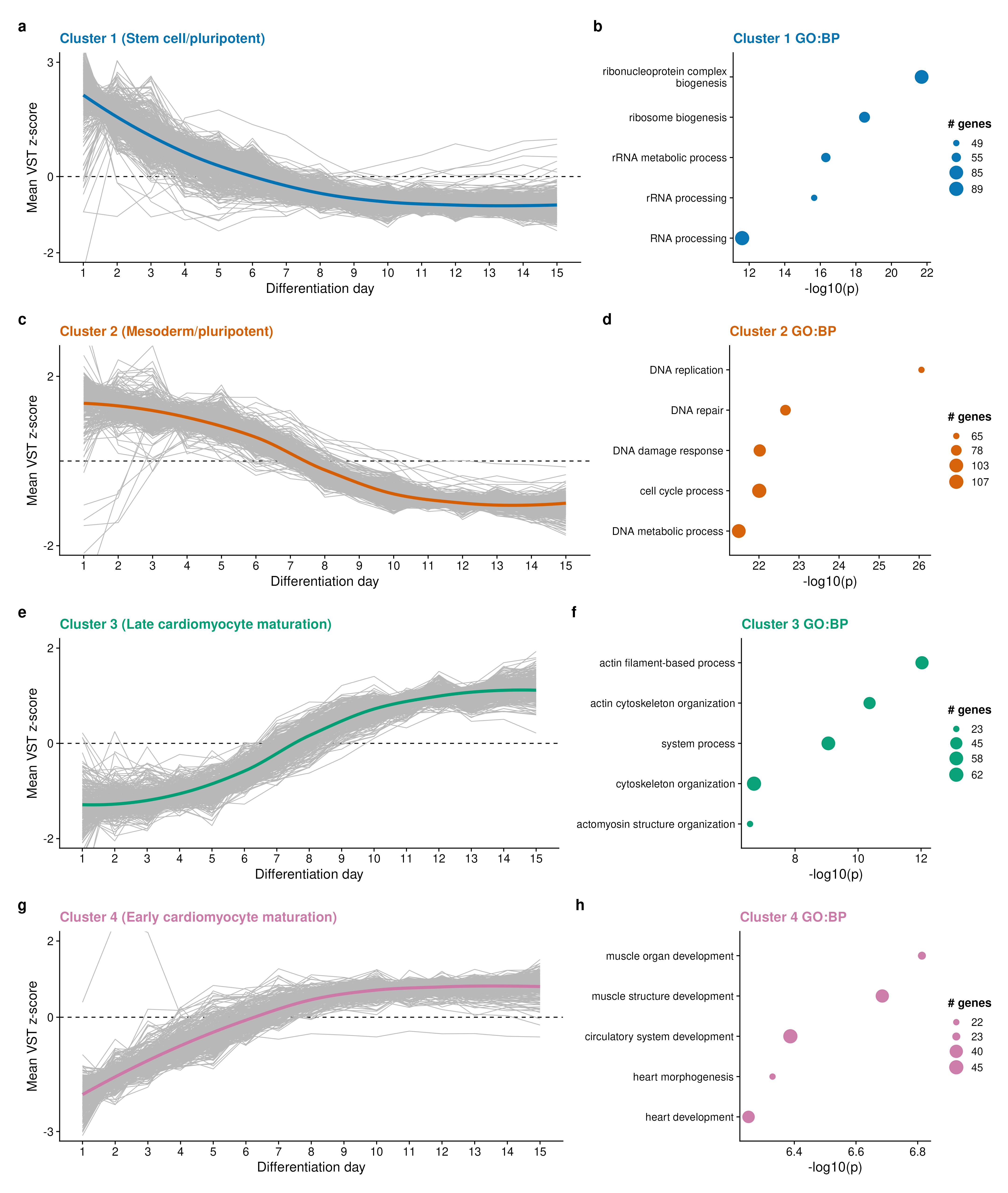
The cluster trajectories summarize expression patterns. They are not additional differentiation scores.

4.2 Fit the PCA reference space

The scorer fits PCA to reference timepoint means, not individual samples. The resulting path represents mean expression at each observed timepoint; within-timepoint variation does not define the path.

Let \(\mathbf{x}_i\) be the normalized expression vector for sample \(i\), restricted to the selected temporal genes. For a reference timepoint \(t\), let \(\bar{\mathbf{x}}_t\) be the mean vector across its reference samples:

\[ \bar{\mathbf{x}}_t = \frac{1}{n_t}\sum_{i:\,t_i=t} \mathbf{x}_i. \tag{1} \]

The function fits centered, unscaled PCA to the collection of \(\bar{\mathbf{x}}_t\) vectors. Let \(\boldsymbol{\mu}\) be the mean of those timepoint means and let \(W\) contain the retained PCA loading vectors. The PCA coordinates for any sample are

\[ \mathbf{z}_i = (\mathbf{x}_i - \boldsymbol{\mu})W. \tag{2} \]

The same transformation maps both reference and non-reference samples into the reference space. In the GSE122380 fit, seven PCs meet the 99% variance target. The number can change when the reference cohort or temporal-gene set changes.

Figure 4. Individual samples projected into centered, unscaled PCA spaces learned from timepoint means for the full temporal set and two cluster subsets. C1+C2 and C3+C4 are shown for comparison, not as alternative models.

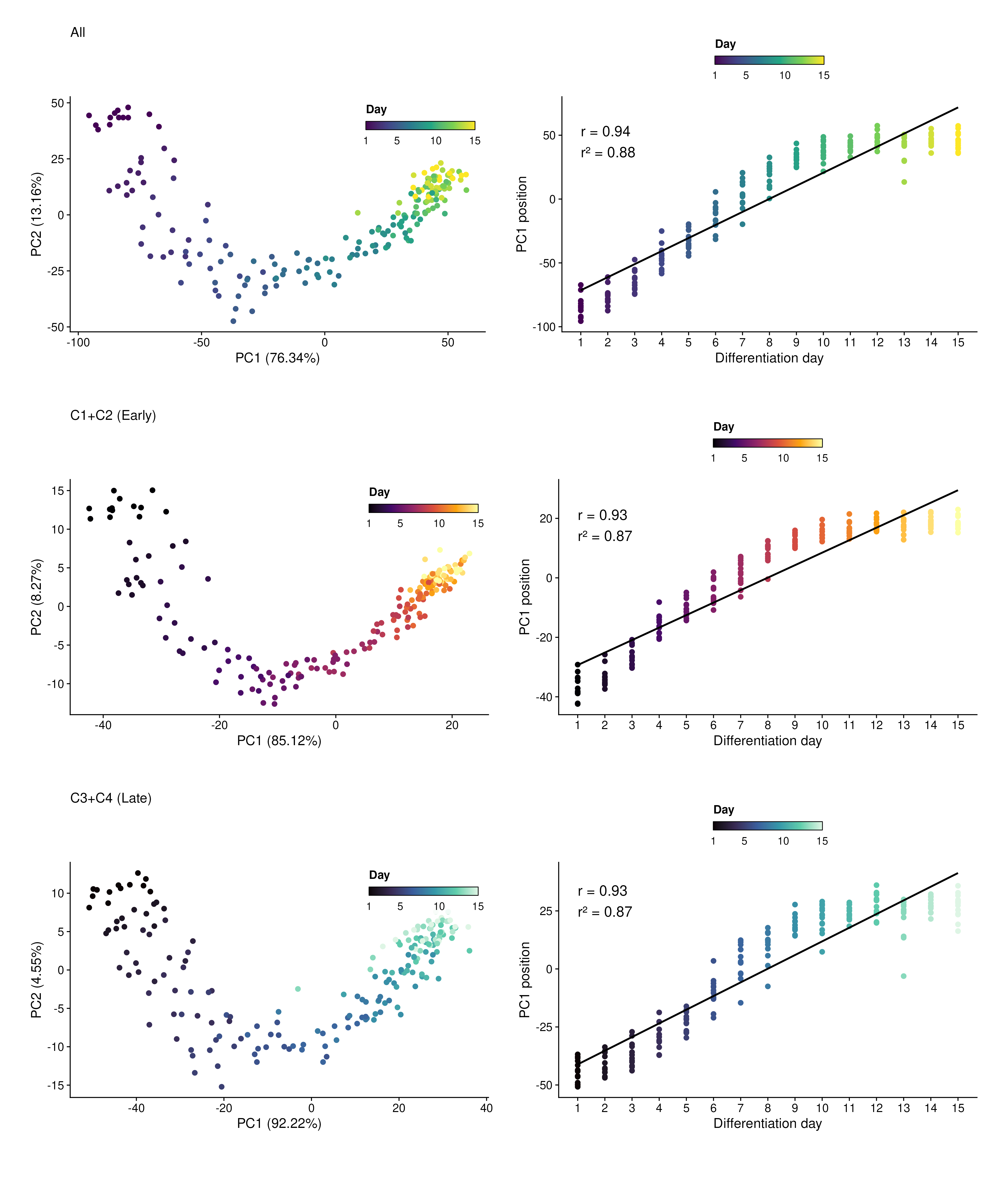
The full temporal-gene panel shows the PCA space used for scoring. The cluster panels show how selected expression subsets relate to the same time course; they do not replace the full temporal-gene model.

Use PCA loadings to inspect which genes contribute to the reference axes. Figure 5 labels the largest PC1 and PC2 loadings and tests the strongest PC1 loadings for GO enrichment. The enrichment annotates the PCA axes; it is not part of the timing score.

Figure 5. PCA loading genes and GO enrichment. a-b. The ten largest positive and negative PC1 and PC2 loading genes. Ambiguous Ensembl-to-symbol mappings retain the Ensembl ID. c-d. GO enrichment among the 500 strongest negative and positive PC1 loadings.

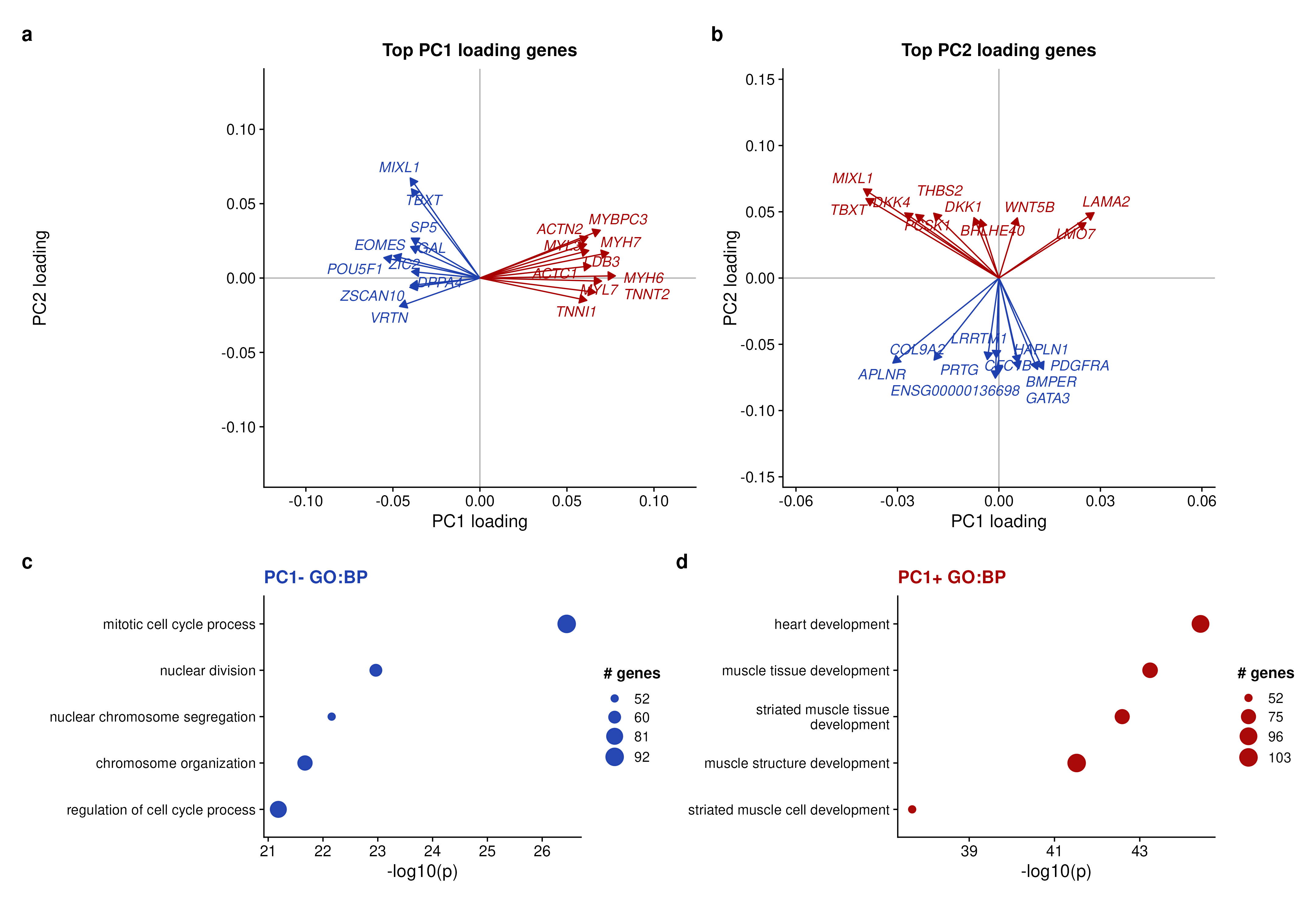
The sign of a PCA axis is arbitrary. The build flips PC1 for figure readability when needed, but this does not change Euclidean distances or sample scores.

4.3 Build and score the reference trajectory

The scorer converts the ordered reference timepoint means into centroids in the retained PCA space. Adjacent centroids define finite line segments. A sample can therefore follow a path that bends across several PCs instead of being ranked by PC1 alone.

For one segment, let \(\mathbf{a}\) and \(\mathbf{b}\) be its start and end centroids, and let \(\mathbf{z}\) be a sample’s PCA coordinate. The segment direction is \(\mathbf{v}=\mathbf{b}-\mathbf{a}\). The closest point on the finite segment is

\[ \alpha = \operatorname{clip}_{[0,1]} \left( \frac{\langle \mathbf{z}-\mathbf{a},\mathbf{v}\rangle} {\langle \mathbf{v},\mathbf{v}\rangle} \right), \qquad \mathbf{q}=\mathbf{a}+\alpha\mathbf{v}. \tag{3} \]

The clipping keeps \(\alpha\) between 0 and 1, so the projection stays on the segment rather than extending beyond a reference endpoint. The scorer evaluates every segment and uses the one with the smallest squared distance \(\lVert\mathbf{z}-\mathbf{q}\rVert^2\). It then interpolates time along that segment:

\[ \widehat{t}=t_a+\alpha(t_b-t_a), \qquad s=\frac{\widehat{t}-t_{\min}}{t_{\max}-t_{\min}}. \tag{4} \]

Here \(t_a\) and \(t_b\) are the segment endpoint times. The score is 0 at the earliest reference time and 1 at the latest reference time. Because the projection is clipped to finite segments, the reported time stays within the reference time range.

Zero-length segments are omitted. A trajectory that folds back near itself can produce ambiguous nearest-segment assignments; review squared distance and the trajectory plot when adapting the method.

source('functions/score_differentiation_timing.R')

timing_fit <- score_differentiation_timing(
  expression_matrix = vst,
  metadata = metadata,
  temporal_genes = temporal_genes,
  sample_id_col = 'sample_id',
  time_col = 'day_numeric'
)

timing_fit$scores[, c(
  'sample_id',
  'observed_time',
  'predicted_time',
  'differentiation_score',
  'squared_distance'
)]

Figure 6 shows the fitted path in the first two PCs. The path is defined in all retained PCs; the figure is a two-dimensional view.

Figure 6. Differentiation trajectory in reference PCA space. Black points are day centroids; arrows connect them in day order. The day 1 and day 15 centroids anchor scores 0 and 1.

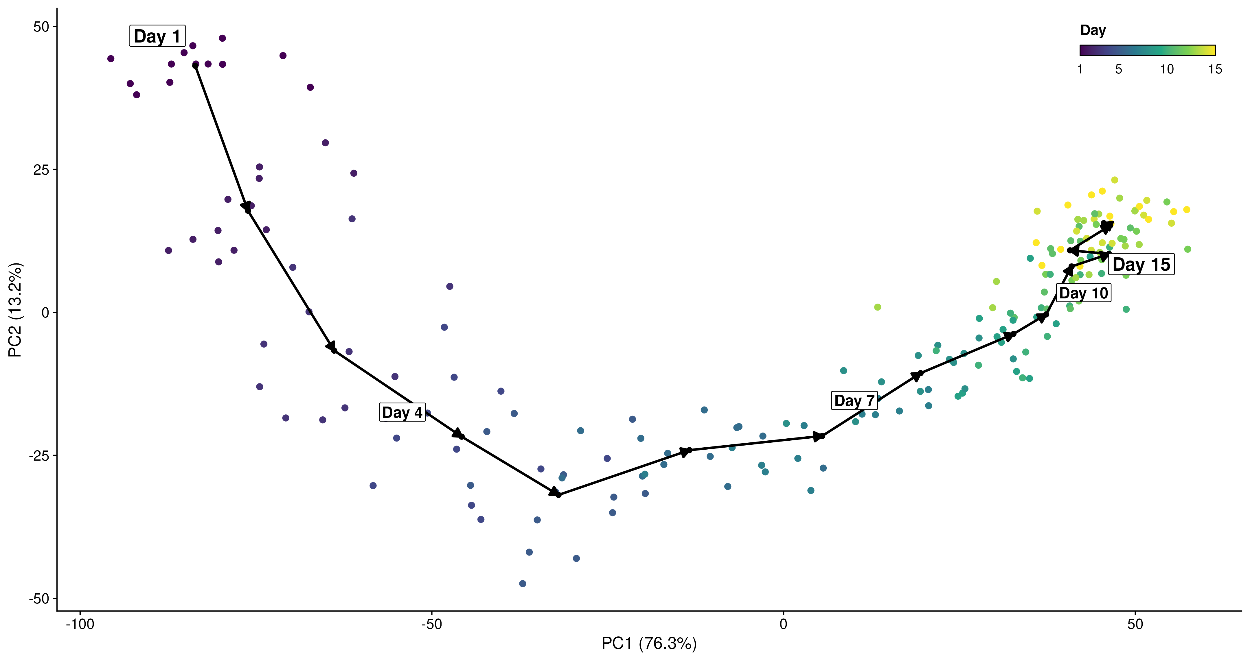
The centroids define the reference path. The path is not a single-axis ranking and does not assume that the samples move at a constant rate between observed timepoints.

Figure 7 shows the scores of the reference samples projected back onto the fitted path. This is a calibration view because the same reference samples define the PCA and trajectory.

Figure 7. Reference-sample differentiation timing scores by observed day. Dashed lines mark the bounded reference endpoints at 0 and 1.

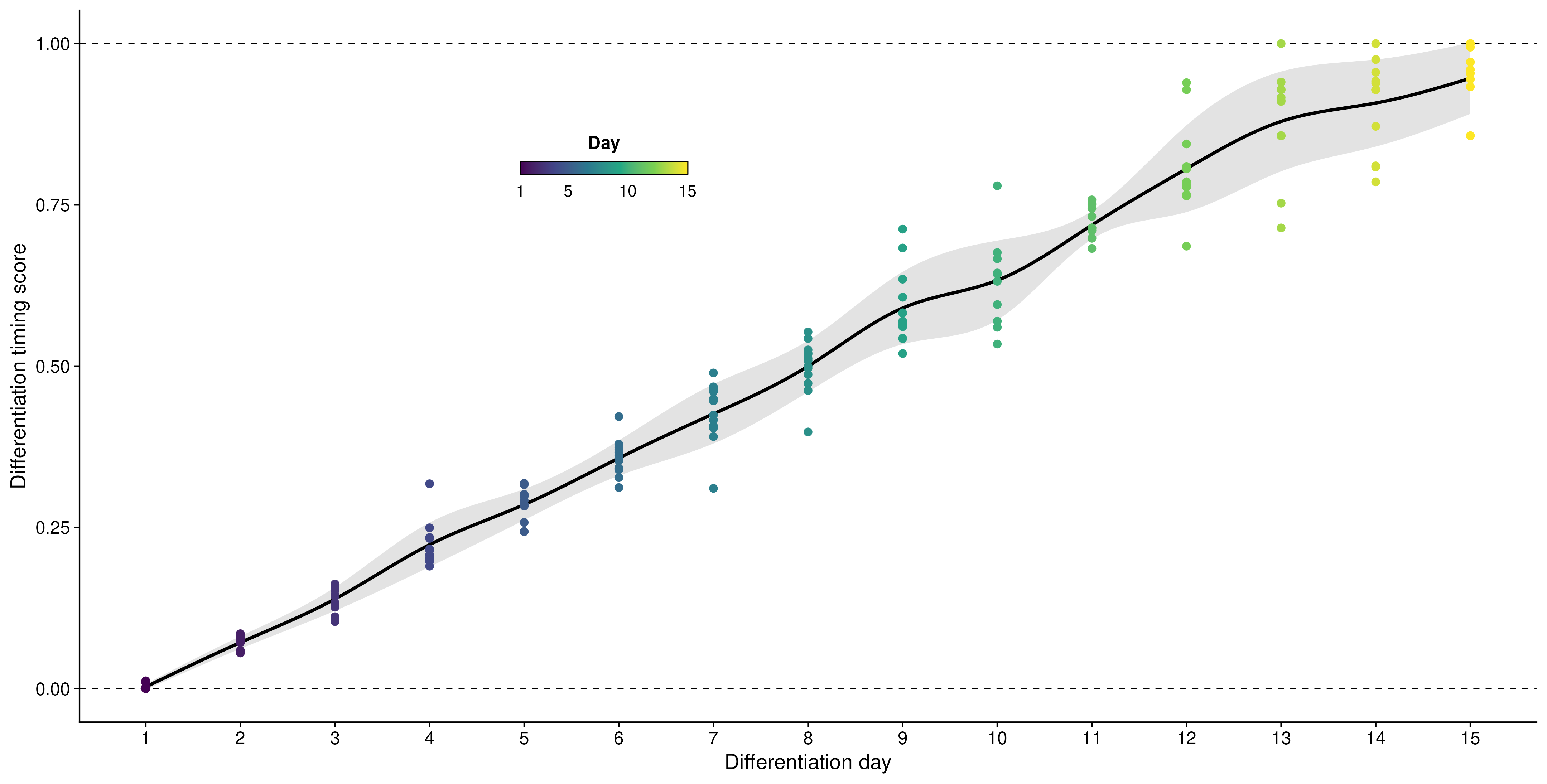
The spread within a day shows how much samples differ around the reference trajectory. It is not an out-of-sample accuracy estimate.

5 Leave-one-out validation of maturation score

The validation tests whether a trajectory trained without one cell line can predict the samples from that cell line. For each held-out cell line, the workflow:

1. removes that cell line from the training reference;
2. selects temporal genes using the remaining cell lines;
3. fits the PCA and centroid trajectory using the remaining cell lines; and
4. projects the held-out samples onto that fitted trajectory.

The count-based DESeq2 LRT is refit in every fold. The tracked VST matrix is shared across folds because the upstream VST transformation is not available in the repository. The validation therefore measures internal transfer within this processed cohort, conditional on the tracked VST matrix. It is not an external validation study.

The validation function also labels fold-specific genes as maturation or progenitor genes according to the sign of their Spearman correlation with time. Those labels annotate genes only. The reported accuracy metrics use the complete temporal-gene set.

source('functions/get_temporal_genes.R')
source('functions/score_differentiation_timing.R')
source('functions/run_loo_maturation.R')

loo_validation <- run_loo_maturation(
  counts = counts,
  vst = vst,
  metadata = metadata
)

loo_validation$summary

All 13 cell lines contribute to the validation. Cell line 19190 is omitted only from the per-cell-line figure to keep the display at 3 by 4 panels.

Table 5.1: Leave-one-cell-line-out validation summary.

Metric	Value
Held-out cell lines	13
Held-out samples	192
Correlation between actual and predicted day	0.979
Squared Pearson correlation	0.959
Mean absolute error	0.55 days
Median absolute error	0.30 days
Predictions within 1 day	82.3%
Predictions within 2 days	97.9%

In this reference, held-out predictions correlate 0.979 with observed days. The median absolute error is 0.30 days, and 82.3% of predictions are within one day. These values describe this cohort and this processing pipeline; they are not universal performance guarantees.

Figure 8. Held-out predictions for 12 displayed cell lines. Each panel reports Pearson \(r\) and its square for that line; neither quantity is a predictive \(R^2\) statistic.

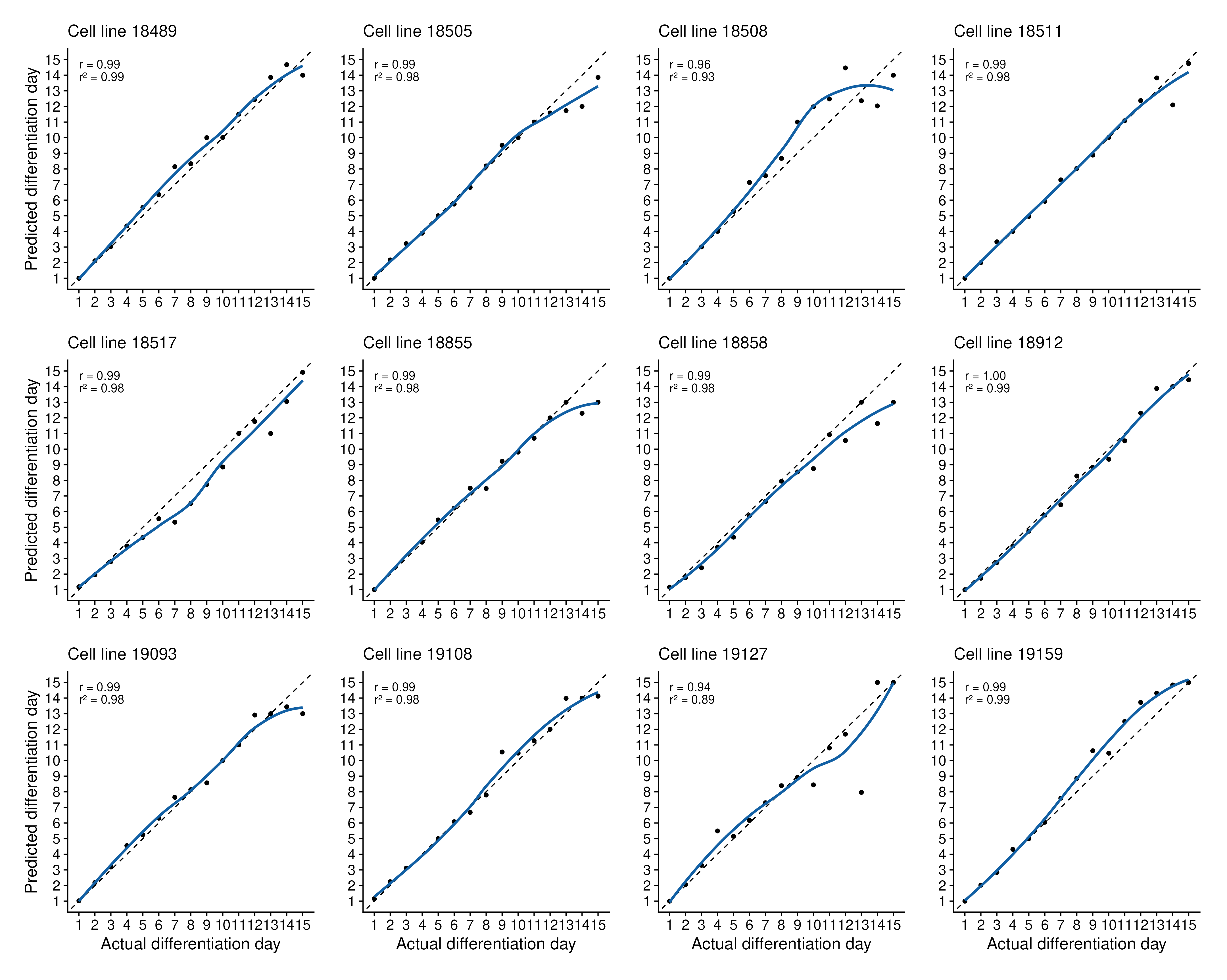
Performance varies across cell lines. Review the per-cell-line panels when deciding whether the reference cohort represents a new study.

Figure 9. Predicted versus observed differentiation day for all held-out samples. The dashed line is identity; the solid line is an ordinary least-squares summary.

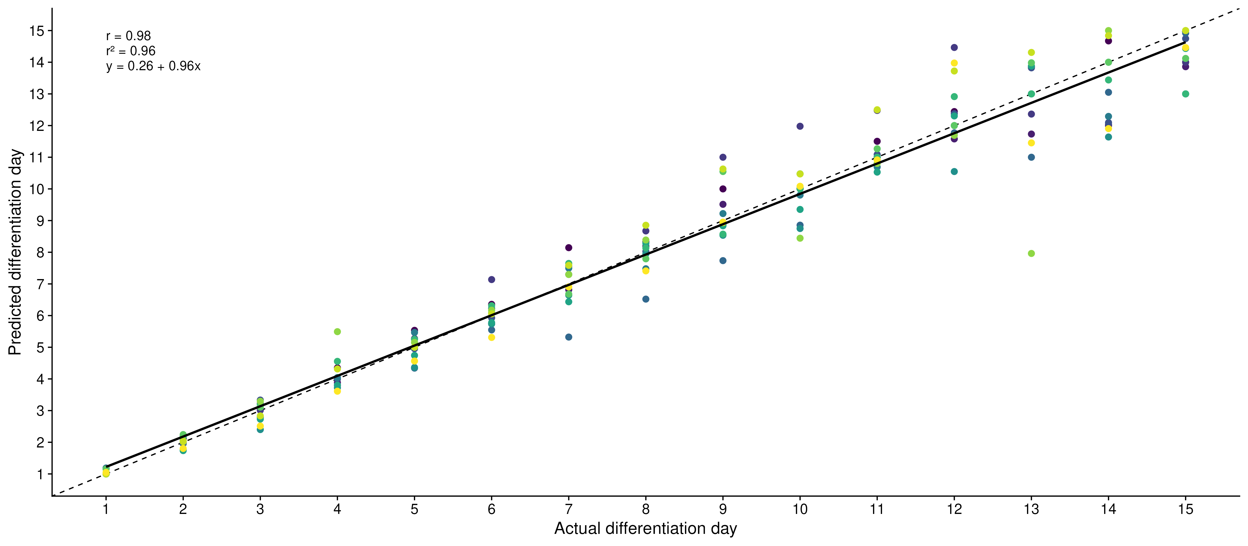
The identity line represents exact timing prediction. The fitted line summarizes association in this cohort; it does not replace the sample-level error measures.

For held-out sample \(i\), absolute prediction error is

\[ e_i = |\widehat{t}_i - t_i|. \tag{5} \]

Figure 10 summarizes the mean absolute error at each observed day. The error bars show one standard deviation across held-out samples at that day.

Figure 10. Absolute held-out prediction error by day. Lower values indicate closer timing predictions.

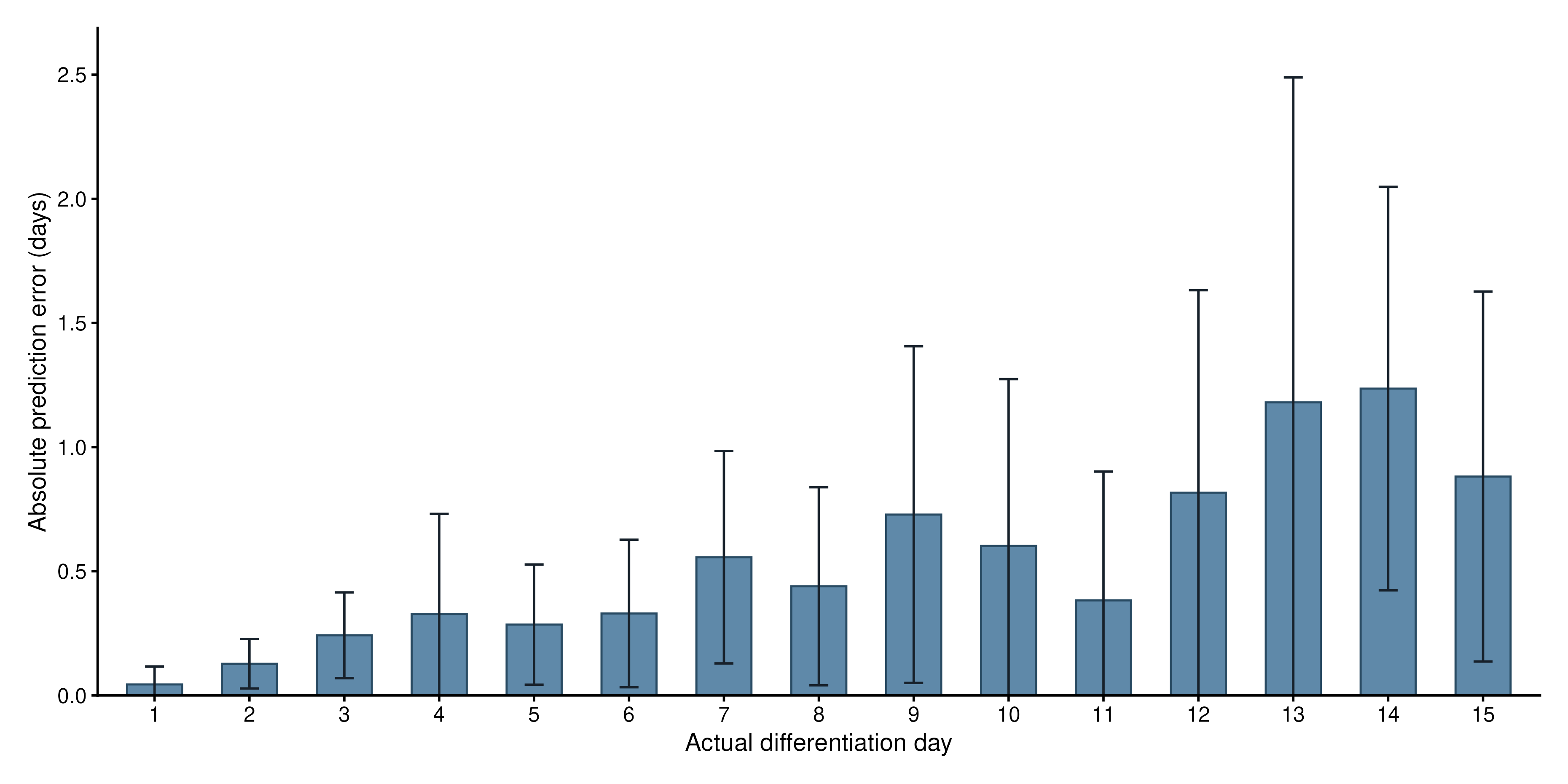
Compare day-specific errors with the overall summary when assessing the reference time course.

6 Interpreting results

6.1 Interpreting scores

Use the sample-level timing_fit$scores table to read the result:

• predicted_time gives the sample’s position on the original reference-time scale.
• differentiation_score rescales that position so the earliest and latest reference times are 0 and 1.
• squared_distance measures how close the sample is to its nearest trajectory segment in the retained PCA space.

The score is relative to the selected reference. A score of 0.5 means that the predicted time is halfway between the earliest and latest reference times after endpoint scaling; it does not mean that the sample has reached half of an absolute biological process. Read squared distance with the score. A large value means that the sample is far from the learned reference path; compare it with reference-sample distances before interpreting the score.

6.2 Adapting maturation score

Use an independent reference cohort with known timepoints to select temporal genes and fit the trajectory. Then project new samples without refitting the PCA or temporal-gene set on those samples. Pass the reference sample IDs through reference_samples:

timing_fit <- score_differentiation_timing(
  expression_matrix = expression_matrix,
  metadata = metadata,
  temporal_genes = temporal_genes,
  reference_samples = reference_sample_ids
)

Before comparing scores, check that gene identifiers and sample identifiers match, expression values use the same normalization convention, and the reference spans the relevant time range. Compare new-sample squared distances with the reference-sample distances. If the biological process or batch structure differs from the reference, fit a new reference model rather than treating the score as directly comparable.

7 References

1. Love MI, Huber W, Anders S. Moderated estimation of fold change and dispersion for RNA-seq data with DESeq2. Genome Biology. 2014;15:550. doi:10.1186/s13059-014-0550-8
2. Robinson MD, McCarthy DJ, Smyth GK. edgeR: a Bioconductor package for differential expression analysis of digital gene expression data. Bioinformatics. 2010;26(1):139–140. doi:10.1093/bioinformatics/btp616
3. Strober BJ, Elorbany R, Rhodes K, et al. Dynamic genetic regulation of gene expression during cellular differentiation. Science. 2019;364(6447):1287–1290. doi:10.1126/science.aaw0040
4. NCBI GEO accession GSE122380

8 Session information

## R version 4.6.1 (2026-06-24)
## Platform: aarch64-apple-darwin23
## Running under: macOS Tahoe 26.5.1
## Matrix products: default
## BLAS:   /Library/Frameworks/R.framework/Versions/4.6/Resources/lib/libRblas.0.dylib
## LAPACK: /Library/Frameworks/R.framework/Versions/4.6/Resources/lib/libRlapack.dylib;  LAPACK version 3.12.1
## locale:
## [1] C.UTF-8/C.UTF-8/C.UTF-8/C/C.UTF-8/C.UTF-8
## time zone: America/Chicago
## tzcode source: internal
## attached base packages:
## [1] grid      stats4    stats     graphics  grDevices utils     datasets
## [8] methods   base
## other attached packages:
##  [1] viridis_0.6.5               viridisLite_0.4.3
##  [3] systemfonts_1.3.2           scales_1.4.0
##  [5] ragg_1.5.2                  patchwork_1.3.2
##  [7] org.Hs.eg.db_3.23.1         ggrepel_0.9.8
##  [9] ggplot2_4.0.3               edgeR_4.10.1
## [11] limma_3.68.4                DESeq2_1.52.0
## [13] SummarizedExperiment_1.42.0 MatrixGenerics_1.24.0
## [15] matrixStats_1.5.0           GenomicRanges_1.64.0
## [17] Seqinfo_1.2.0               ComplexHeatmap_2.28.0
## [19] clusterProfiler_4.20.0      circlize_0.4.18
## [21] AnnotationDbi_1.74.0        IRanges_2.46.0
## [23] S4Vectors_0.50.1            Biobase_2.72.0
## [25] BiocGenerics_0.58.1         generics_0.1.4
## [27] bookdown_0.47
## loaded via a namespace (and not attached):
##   [1] RColorBrewer_1.1-3      rstudioapi_0.19.0       jsonlite_2.0.0
##   [4] shape_1.4.6.1           tidydr_0.0.6            magrittr_2.0.5
##   [7] magick_2.9.1            ggtangle_0.1.2          rmarkdown_2.31
##  [10] farver_2.1.2            GlobalOptions_0.1.4     fs_2.1.0
##  [13] vctrs_0.7.3             Cairo_1.7-0             memoise_2.0.1
##  [16] ggtree_4.2.0            htmltools_0.5.9         S4Arrays_1.12.0
##  [19] SparseArray_1.12.2      gridGraphics_0.5-1      sass_0.4.10
##  [22] bslib_0.11.0            htmlwidgets_1.6.4       plyr_1.8.9
##  [25] httr2_1.3.0             cachem_1.1.0            igraph_2.3.3
##  [28] lifecycle_1.0.5         iterators_1.0.14        pkgconfig_2.0.3
##  [31] Matrix_1.7-5            R6_2.6.1                fastmap_1.2.0
##  [34] gson_0.2.0              clue_0.3-68             digest_0.6.39
##  [37] aplot_0.3.1             enrichplot_1.32.0       colorspace_2.1-3
##  [40] ggnewscale_0.5.2        aisdk_1.4.12            textshaping_1.0.5
##  [43] RSQLite_3.53.3          labeling_0.4.3          mgcv_1.9-4
##  [46] abind_1.4-8             httr_1.4.8              polyclip_1.10-7
##  [49] compiler_4.6.1          bit64_4.8.2             fontquiver_0.2.1
##  [52] withr_3.0.3             doParallel_1.0.17       S7_0.2.2
##  [55] BiocParallel_1.46.0     DBI_1.3.0               ggforce_0.5.0
##  [58] R.utils_2.13.0          MASS_7.3-65             DelayedArray_0.38.2
##  [61] rappdirs_0.3.4          rjson_0.2.23            tools_4.6.1
##  [64] otel_0.2.0              ape_5.8-1               scatterpie_0.2.6
##  [67] R.oo_1.27.1             glue_1.8.1              callr_3.8.0
##  [70] nlme_3.1-169            R.cache_0.17.0          GOSemSim_2.38.3
##  [73] cluster_2.1.8.2         reshape2_1.4.5          gtable_0.3.6
##  [76] R.methodsS3_1.8.2       tidyr_1.3.2             XVector_0.52.0
##  [79] foreach_1.5.2           pillar_1.11.1           stringr_1.6.0
##  [82] yulab.utils_0.2.4       splines_4.6.1           dplyr_1.2.1
##  [85] tweenr_2.0.3            treeio_1.36.1           lattice_0.22-9
##  [88] bit_4.6.0               tidyselect_1.2.1        locfit_1.5-9.12
##  [91] fontLiberation_0.1.0    GO.db_3.23.1            Biostrings_2.80.1
##  [94] knitr_1.51              gridExtra_2.3.1         fontBitstreamVera_0.1.1
##  [97] xfun_0.60               statmod_1.5.2           stringi_1.8.7
## [100] lazyeval_0.2.3          ggfun_0.2.1             yaml_2.3.12
## [103] evaluate_1.0.5          codetools_0.2-20        gdtools_0.5.1
## [106] tibble_3.3.1            qvalue_2.44.0           BiocManager_1.30.27
## [109] ggplotify_0.1.3         cli_3.6.6               jquerylib_0.1.4
## [112] processx_3.9.0          styler_1.11.0           dichromat_2.0-0.1
## [115] Rcpp_1.1.2              png_0.1-9               parallel_4.6.1
## [118] blob_1.3.0              DOSE_4.6.0              tidytree_0.4.8
## [121] ggiraph_0.9.6           enrichit_0.2.0          purrr_1.2.2
## [124] crayon_1.5.3            GetoptLong_1.1.1        rlang_1.3.0
## [127] KEGGREST_1.52.2